What is HypoSite?

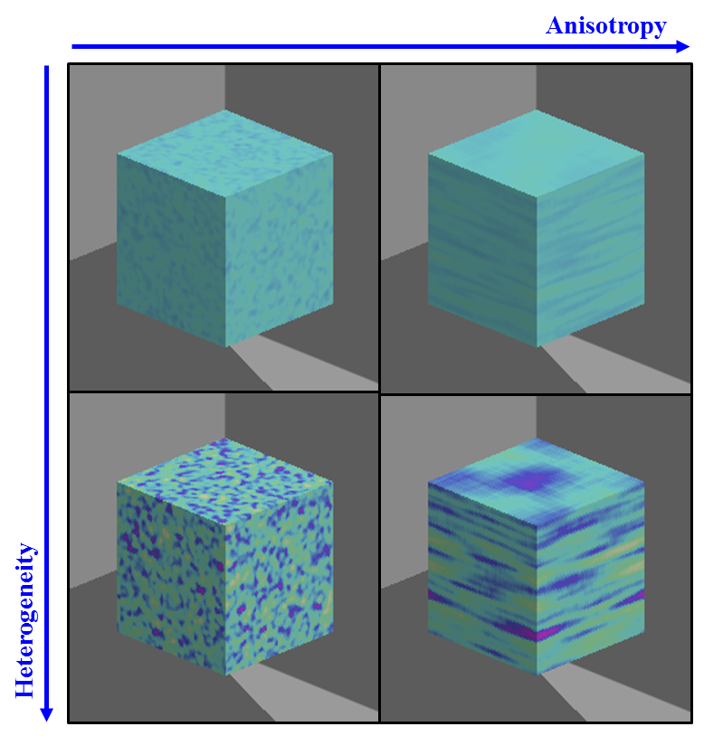
Is it possible to test if a model is correct? Ask yourselves, first: What does “correct” mean? What does “model” mean? The latter can be debated for ages with no success, everyone I have encountered in the business has a perfectly clear view of what a model is, and they all differ. Most of them are right though…For an exposé, have a look at the excellent paper on the issue by Nordstrom.

How many papers have you seen in which “models” are “validated” against real “data”? Can a model even be “validated”? The clear and easy answer is simply no! Karl Popper argued that the induction approach to science, which emanated from the Renaissance era, should be repudiated. Instead Popper argued for “falsification”. With this is meant that a model can be proven wrong, but never proven to be right. So if we believe in Popper, our task is to try to prove a model wrong. If we fail, after hard work, then probably our model is not very wrong, at least for the moment.

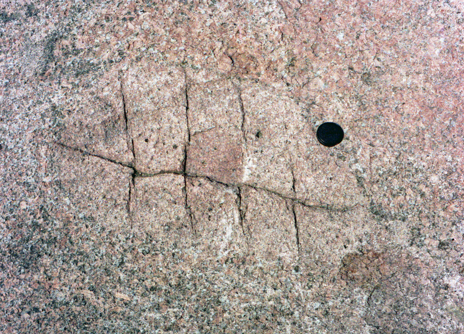
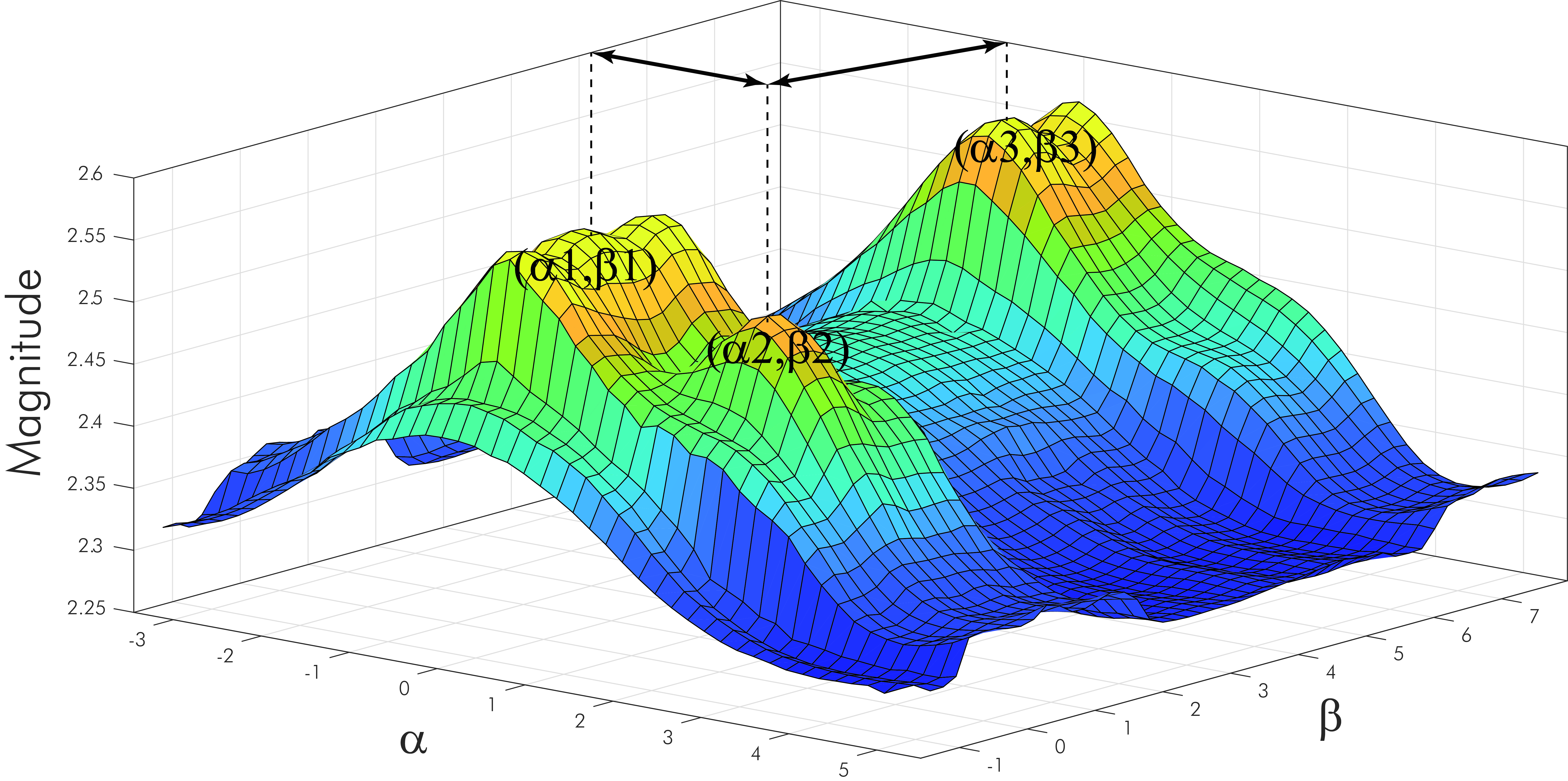
So how do we test if a model is wrong? Well, that is actually fairly easy. If it fails to predict what we know is right, within reasonable bounds, then it is simply wrong! But how do we know what is right? Certainly not by comparing to samples from the real world with all their biases, intrinsic variability, resolution issues, instrumental imprecision, human errors, etc.

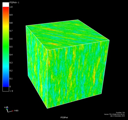
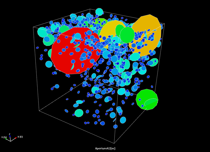
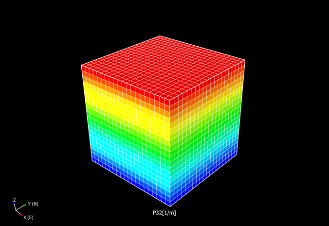
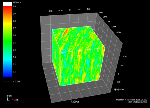
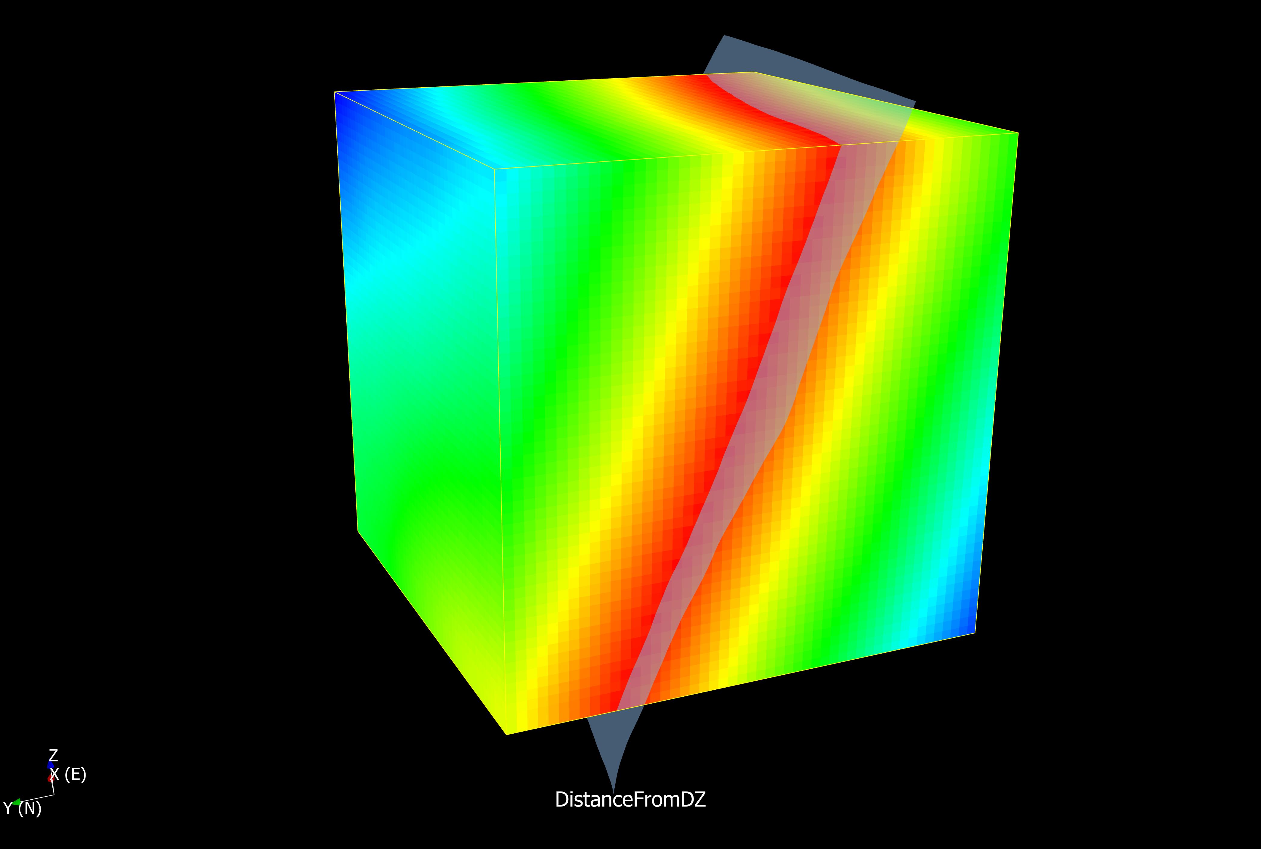
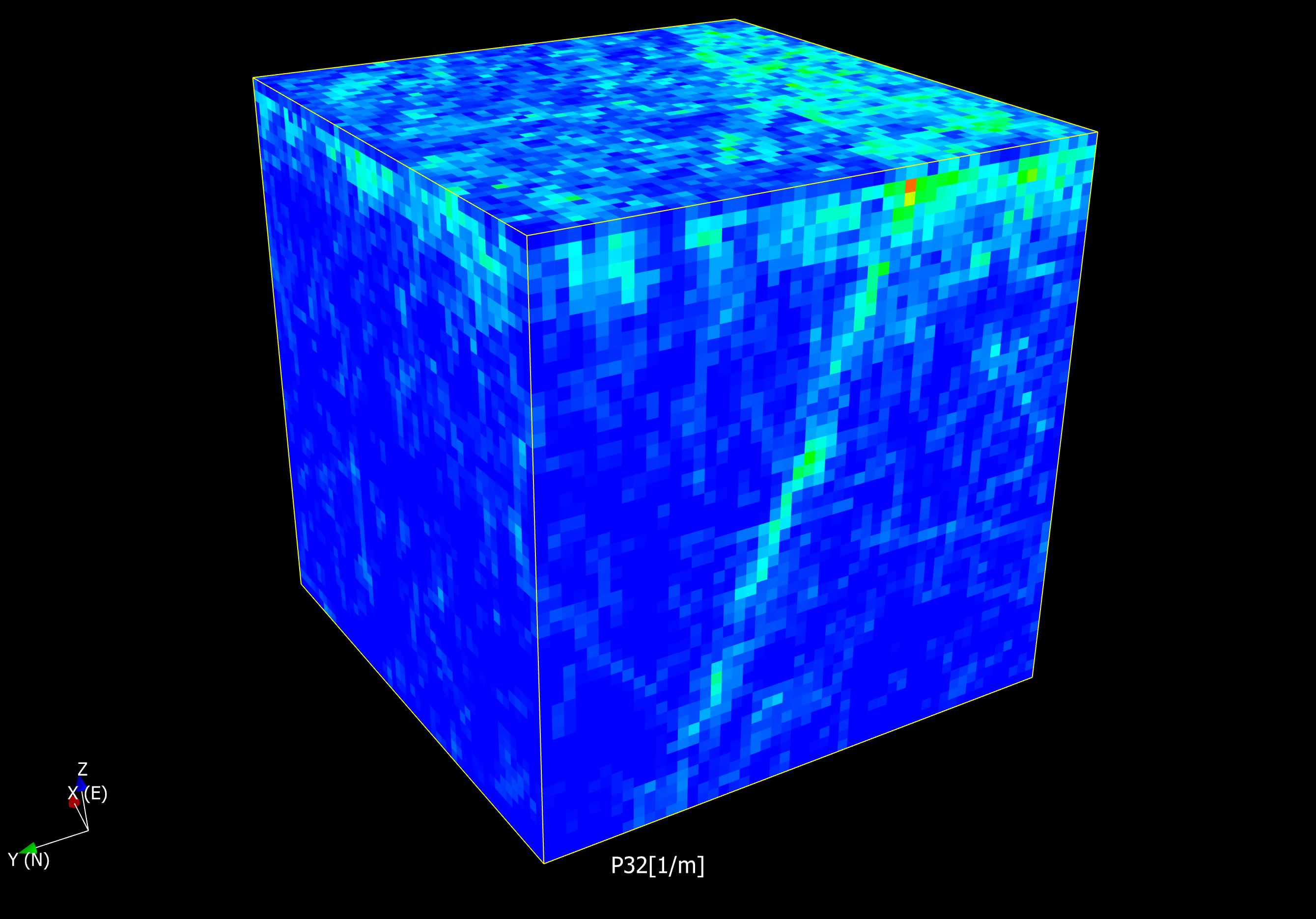
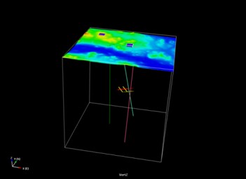
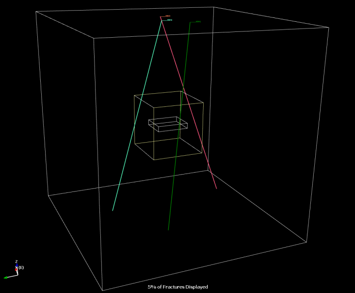
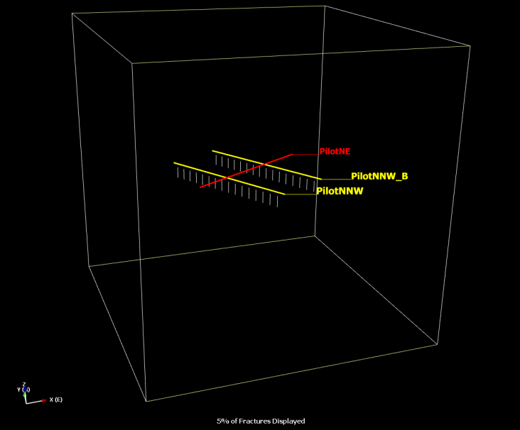
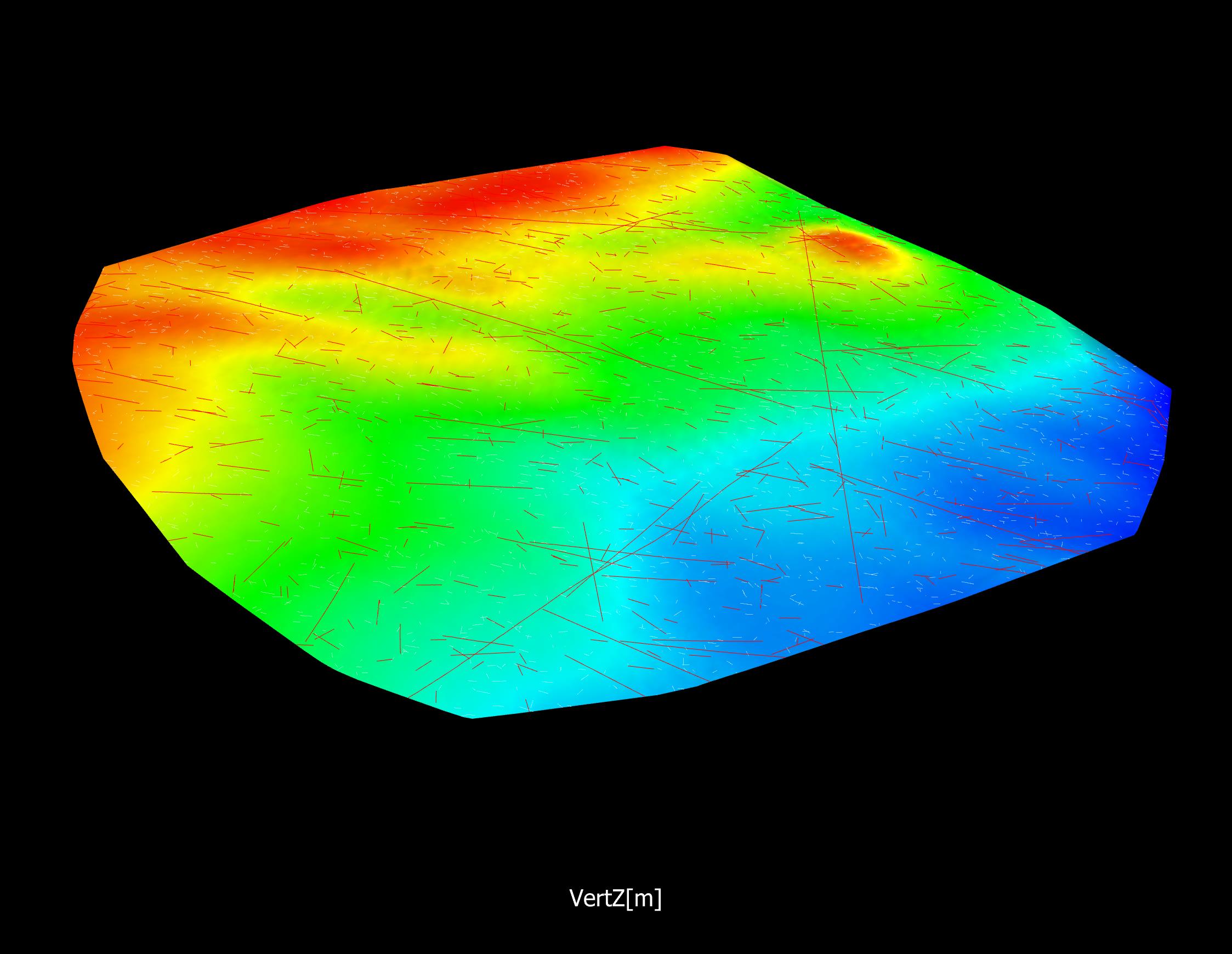
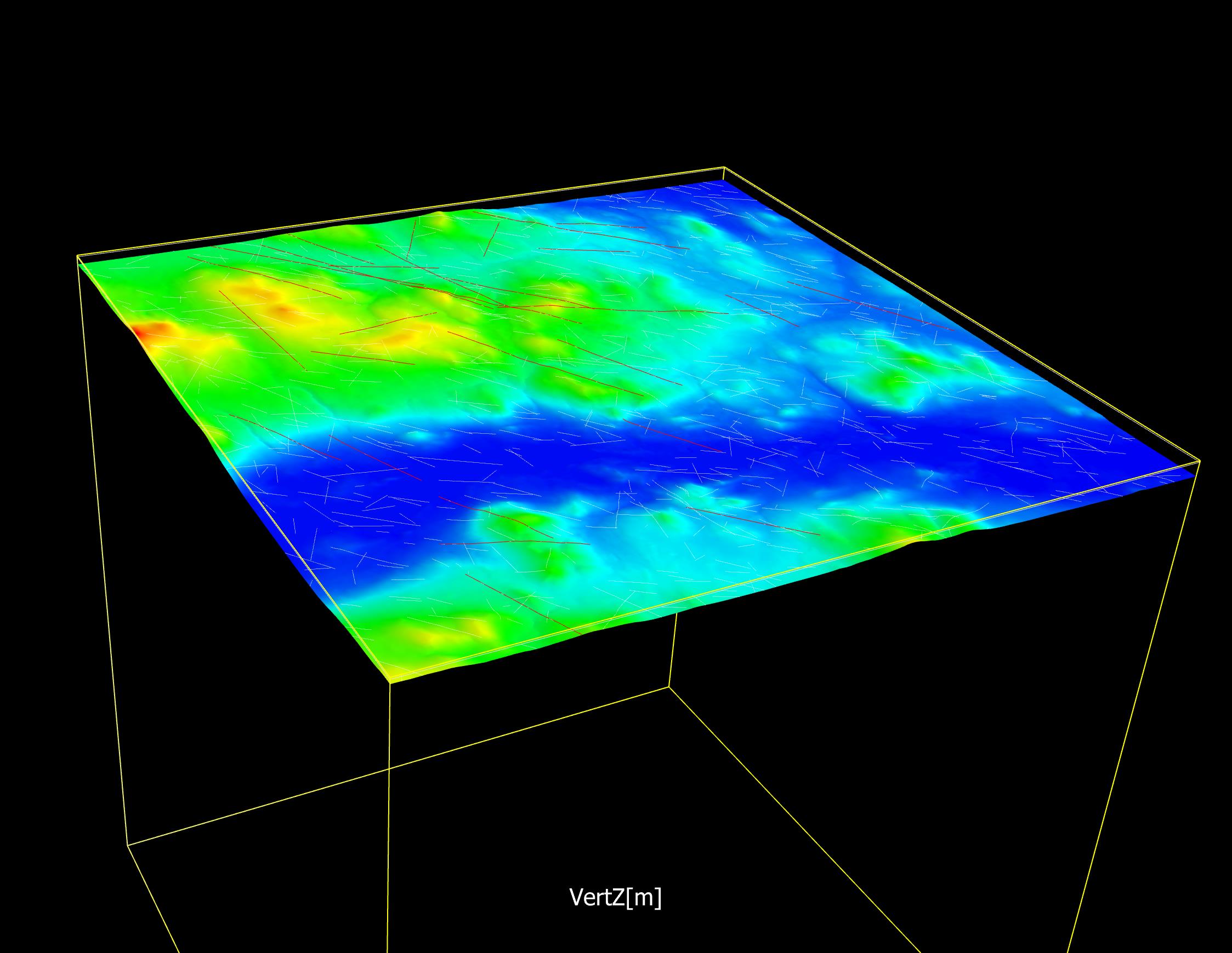
The only way to know what is right, without any doubt and full control over all variability, is to construct the reality against which we test our model. If we fail to replicate what we know is right, we need to iterate the modelling procedure, reassess our assumptions, tweek parameters and so on until we succeed. Thereafter we might apply our codes to real data and hope that our model is not too wrong. Given, of course, that our artificial data is sufficiently close to the reality we aim our modelling efforts towards.

HypoSite offers just that. It is an acronym for Hypothetical Site(s) which is:

- A collection of controlled geological settings handcrafted in our laboratory.
- A collage of controlled data sets, stemming from the artificial realities, as input to testing DFN codes and concepts.

The main purpose is to provide a tool for bench-marking codes and concepts, evaluate methodologies and test new implementations of codes. It was originally intended to all aspects of geology, but it is, for the moment, focused mainly on the DFN aspect of geological modelling.

Who would need HypoSite?

Those of us who wish to:

- Compare different DFN tools and concepts,
- Test new algorithms in DFN tools.

Basic principles

We construct test cases as a collage of hypothetical data sets with Perfectly known geometries and parameters.

- We mimic real world applications. Therefore the test cases need to be realistic.
- Each ”test case” is deterministic (a “frosen”, single, realisation).
- The “recipe” is stochastic (a set of statistical distributions, rules assumptions).
- We extract samples from artificial boreholes, tunnels and outcrops which makes intersections with the structures and formations within HypoSite, and use these as input to the DFN tools, thereby mimicking real “data”.
- We start very simple, and add complexities as we progress with the tools. We construct a Base Model (BM) with variants of increasing complexities
- To ensure realism, we base our models on real data

Homogeneity and anisotropy

Anisotropy/homogeneity is steered by:

Intensity (P32), Size distribution, Orientation, Size + P32, Orientation + P32, Size + orientation, Orientation + size + P32.

Note, different parts of a model (domains) can contain aspects from each of these end member.

For one and the same intensity, there is an infinite number of size distributions to choose from which will steer the number of fractures in the model. In other words, intensity and size are intimately correlated.

The intensity can be random (Poisson)

The intensity can be an isotropic fractal

The intensity can be an anisotropic fractal, mimicking fracture swarms or deformations zones

Aperture

Assumption #1: There are 2 main categories of fractures: Open and sealed.

Open fractures are (more or less) open over their entire surface. They constitute a specific subset of the network and are hence not any artifact of sampling.
Sealed fractures are sealed over their entire surface

Assumption #2: All fractures are open, at least at some part on their surface. The amount of void, and the spatial distribution of the voids, can be expressed by statistical distributions.

We further assume that the aperture can be described by a distribution and that the aperture distribution is a function of stress field (present and past) and God knows what.
The maximum aperture is a function of the fracture size. That is, the aperture distribution itself scales with fracture size.

Mechanical aperture seems to scale linearly with radius for faults

Mechanical aperture seems to scale powerlaw with radius for Mode I (pure opening) fractures. So what shall we use? It is not really important as long as apertures gives fairly “realistic” flows in our mode, i.e. fairly well mimic what we measure in field. We create both the fractures and the flow so we will still have perfect control over our own “reality” which is the purpose of HypoSite.

Proposal: Compute average aperture according to Klimczak

equ 7, thereby assuming fractures with modes ≥ I.

We assume aperture according to Klimczak et al (2010).

The parameter “α” can be either a constant or a distribution. A Gaussian distribution will tend to a lognormal-type distribution of apertures whereas a constant yields a powerlaw.

We assume a transmissivity of the type Zimmerman & Bodvarsson, 1996.

Assumption #1.

Some fractures are closed. The smaller the radii, the higher probability of beeing closed.

Assumption #2.

All fractures are open. Aperture is function of size (with some randomness).

Two apertures are computed for each fracture: ApertureA1 and Aperture A2. These correspond to assumptions #1 and #2.

Accordingly, two transmissivities are computed, Transmissivity_A1 and Transmissivity_A2.

The parameter “α” is a random variable.

Trends

The most obvious trend is decreasing intensity of fractures with depth. In analogue, the aperture and transmissivity may too be modeled to decrease with depth. Or to change towards a fault, or both superimposed.

Clustering

Data suggest fractal, anisotropic clusters. Perhaps correlated to lithology, which can be fractal in 3D space.

Fractures can cluster into zones.

fracture swarms or deformations zones can be mimicked by using anisotropic fractal intensity.

Termination

Termination is a function of geologic evolution. But what rules to apply? Older fractures generally longer, i.e. put genesis in the model to mimic an evolution?

We use the idea presented by Davy et al (2013), in which short fractures terminates against larger ones.

The degree of termination can be different for each “age-set”, “orientation.set”, “mineralogical-set”, etc.

Shapes

Different DFN tools support different shapes.
Almost none support 3D geometries (e.g. undulating sheets of variable thickness).

Few support 2.5 D geometries (e.g. undulating surfaces, zero thickness)

Assumptions:

-Truncated/terminated fractures are polygonal (more or less).

-Isolated fractures do not take part of the “action” so their “original” shape is perhaps unimportant. If small they do not interact, if large they interact and terminate or are terminated against.

Truncation of discs yield other final shapes than truncation of squares.

Scaling

Problematic and difficult issue: What is meant by “scaling”?

- It is now widely recognized that power laws and non-Euclidian geometry provide descriptive tools for fracture systems. A key argument is the (obvious, look at the pictures) absence of characteristic length scales in the fracture patterns (and by inference the growth process). All power law characteristics in nature must have upper and lower bounds.
- Uncritical use of analysis techniques has resulted in inaccurate and even meaningless metrics to quantify and characterise fractures. See e.g. Bonnet et al (2001) for discussion.

What are the implications?

- It is possible describe, and model, fracturing at “all” scales simultaneously. Sometimes referred to as “Tectonic continuum”.
- Size and intensity are intimately related and, moreover, intimately related to the size of the system that is modeled.
- Consider this: How large can a single fracture (plane) be? On one scale (say “regional”) it is a single object, a deformation zone. On another scale (say outcrop) it is a cluster of structures. If we describe the system as a single, continuous distribution over all scales, how can it be a single structure and a cluster of smaller structures at the same time?

The photograph above illustrates the problem. Obviously we need to “upscale” clusters to single objects for modelling purposes. Or perhaps the opposite, downscale single objects to clusters of smaller objects. But how to honour global intensity? Where are the transitions? What is mimicking real processes and what is simply convenient for modelling purposes? Field data from Olkiluto, Finland, suggest that single fractures reach a size of ca maximum 100-150 m (equivalent diameter) before they link and cluster to form larger structures.

Deformation zones

HypoSite deformation zones can either display internal and proximal geometries, e.g. include the damage zone (left figure from Rempe et al, 2013), or be represented as a single, large (deterministic) object.

The zone can modeled as a cluster of fractures.

- Intensity decays away from zone
- Symmetric (base case) or asymmetric
- Connected network through the model
- The large scale DZ-plane is not included, only as “guide” (attractor, optionally fractal) for generation of fractures-Intended to mimic a core and damage zone(s)
- Alternatively, intensity is steered by a P32 propability grid
- Provides more realistic intersections with sampling domains
- Makes geological “sense”

Nested models

Ensures samples mimic real world samples by including intersections from all scales.

- Enables modelling of all scales simultaneously
- Computationally efficient for large models
- Complex to build, hence rigid.

The smallest fracture in each subvolume is indicated in the figure to the left. In short, this implies:

- Boreholes will intersect fractures from [0.038-inf] m
- Outcrop and tunnel will intersect fractures from [0.1-inf]

Fracture Domains

The formalism of fracture domains can be expressed as follows: Fracture domains are expressed in Euclidean space, whereas statistical domains (Darcel et al. 2012) are defined in statistical space. Just like the Euclidian space, familiar to us humans, in which we express proximity in terms of metric distance, the proximity in statistical space is expressed in terms of statistical distance (Dodge 2006). Though this might be perceived as a play on words, this formalism is necessary to differentiate between modelling of domain geometries, which takes place in the Euclidian space, from modelling of statistical domains, which takes place in statistical space. Naturally, these are intertwined, and the workflow is iterative as shown on the figure.

The statistical distance is not only a measure of difference between, say, average values or variance of entities, it also expresses the strength of correlation between these entities. We model in the realm of a multidimensional (statistical) space and the entities might be either random variables or a collage of such, along each axis in this multidimensional statistical space. This might be perceived as somewhat abstract but it simply boils down to properties, familiar to us, which define the genome of each DFN model, namely: Intensity, size, orientation, transmissivity, connectivity, location (Eucledian coordinates) and time to name but a few of the most obvious.

Any multidimensional (statistical or Euclidean) space can be sliced so the result is somewhat comprehensible to humans, by slicing it such that the slice itself lies in one of either 1D, 2D or 3D space, which enables visualisation of complex parameter spaces. In analogy to Euclidian space, locations in the statistical space can be expressed in terms of coordinates. The distances between statistical “points”, “lines” and “surfaces” etc can be computed in essentially the same manner. The example shown on the figure displays the correlation and magnitude of two hypothetical entities a and b respectively. These should be understood as either single properties (e.g. intensity and size) or as a combination of many properties (e.g. size/intensity and orientation/age) expressed as an appropriate metric stemming from investigation data (with or without Euclidian coordinates), assumptions or inferences. In the example shown here, the points (a1,b1) and (a2,b2) are considered statistically close whereas the point (a3,b3) is considered statistically distant in the a-b plane. Naturally the distance can also be computed in the a-b-Magnitude volume and the statistical coordinates are instead expressed as triplets (e.g (a,b,Magnitude)). This notion can be expanded to a statistical space of any dimension but cannot with ease be visualised in any comprehensible manner.

The first iteration in the domain building process is to create volumes based on natural boundaries. In this example two rock domains are separated by a plane representative of the DZ through the model. The near-surface bedrock constitutes a domain by its own.

In more complex models, the deformation zones can constitute domains, in which a separate DFN model can be built.

Example of a HypoSite containing a single DZ.

P32 distribution in a model with no domains, nor zones, but with decaying intensity with depth.

Grids are handy to manipulate DFN parameters. Here a grid is used to separate the volume into the main domains, separated by a DZ.

Each domain can have their own characteristics. Here both domains have decaying intensity with depth but at different rates.

This example shows the resulting P32 for a model containing 2 domains, a DZ and decaying intensities in the domains.

Sampling space (support)

HypoSite contains supports of various shapes, dimensions and orientations. The idea is to use realistic supports to intersect the DFN and from these intersections produce “data” aiming to mimic real-world data, with the fundamental difference that the fracture geometries are perfectly known in HypoSite. The computed intersections are further manipulated to mimic sampling policy, for additional realism.

For example, the intersections can produce mm long traces on the tunnels whereas a typical sampling policy would be to sample all traces above, say, 1 m. Thus the intersections (traces) are deliberately truncated and censored to produce the “public samples”.